What is Dispersion Trading?
Dispersion trading is an ETF/index arbitrage strategy that consists of trading the difference in the volatilities between an ETF/index and its individual stocks. One can set up a dispersion trade by buying straddles on the stocks and selling straddles on the ETF/index. Dispersion trading works, because ETF/indices tend to move less than stocks, opening up chances to profit from these mispricing.
Introduction to Dispersion Trading (Implied Correlation Trading)
Navigating the trading waters of recent option markets has proved a formidable challenge for portfolio managers, whose traditional volatility option strategies have often yielded underwhelming results. Against this backdrop, option dispersion trading has emerged as an outlier, delivering robust performance where other volatility methods have failed. Dispersion trading isn’t just a simple play on numbers; it’s a calculated bet on the volatility gap and correlation difference between index options and the options of individual stocks within that index
Dispersion trading exploits the variance in expected volatility between index options and options on the individual stocks of the index. Generally, the implied volatility in index options is not low enough compared to the implied volatility in stock options. This inconsistency leads to opportunities to benefit from the fluctuating spread.
Why do we love this strategy?
Dispersion trading is a low-risk strategy where you either make a small profit or hit a big jackpot. It’s safe because ETFs and indices usually don’t swing wildly. But if a stock in your trade suddenly jumps or drops due to major news, you could earn a lot from the bet you placed on it. And if nothing much happens in the market, the small profits from your short straddle in the ETF or index trades will cover the costs of your long straddles in the stocks.
A key element of dispersion trading is understanding the concept of Option-Implied Correlations. These correlations offer insights into how closely individual stocks are expected to follow the movements of their broader index. When these correlations are high, it indicates that stocks are likely to move in harmony with the index, presenting fewer opportunities for dispersion trading. On the other hand, when correlations are low, suggesting a greater likelihood of individual stock movements deviating from the index, the conditions become ripe for dispersion trading. This divergence is where the strategy truly shines, providing the openings traders seek to capitalize on.
In recent times, the strategy of dispersion trading has gained traction as traders seek effective ways to generate alpha. Often, the complexity of dispersion trading is exaggerated in literature.
How does Dispersion Trading exactly work?
The volatility of a stock index doesn’t usually swing as wildly as its individual stocks due to a principle called diversification—essentially, not all stocks move up or down in perfect harmony. Because of this, the overall index tends to be steadier.
Now, there’s a tendency for market forces to push up the expected correlation between stocks, making the index seem more volatile than it really is. This leads to the implied volatility of indices versus stocks being inflated. Hedge funds and trading desks spot this as an opportunity: they bet against the index’s volatility while buying the volatility of individual stocks. This strategy, known as dispersion trading, aims to profit from the overestimated volatility of the index.
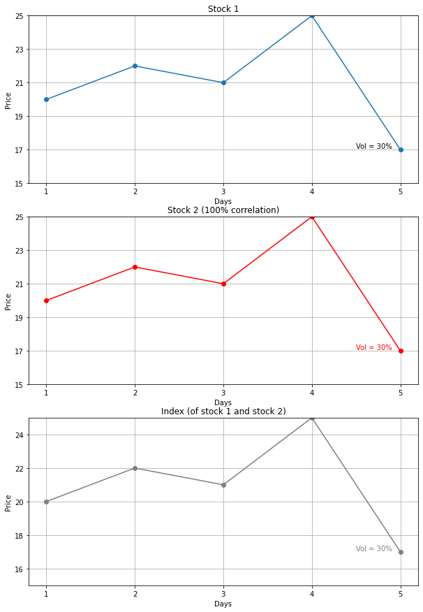
Let’s illustrate with an example. Imagine an ETF/index with just two stocks that move exactly the same way—they’re perfectly correlated (in practise never the case). The index’s ups and downs would exactly match the stocks’. You can see this from the left image below.
Now imagine the opposite case. Imagine these stocks did the opposite of each other, the index wouldn’t move at all—it would have zero volatility, despite the stocks themselves moving quite some around. By being short index straddles and long stock straddles you essentially are making free money. You can see this from the right image. These are the extreme scenario traders look at when they decide where to place their bets. In practise the correlation is somewhere between -100% and 100% (thanks Sherlock).

Dispersion trading is a leading strategy for trading correlations in the market. As stated previously, typically, the expected correlation between stocks, or implied correlation, tends to be overvalued. This is often due to the market positioning of structured product sellers who have a vested interest in going long correlation. This overvaluation makes the implied volatility of indexes appear higher than it actually is when compared to the volatility of individual stocks.
Traders engaging in long dispersion trades aim to take advantage of this by shorting index volatility while simultaneously going long on the volatility of individual stocks. This strategy essentially bets against the prevailing implied correlation. Although dispersion trading is a common way to trade implied correlation, it’s important to note that the success of this strategy is also tied to overall volatility levels. One is essentially trading the index correlation, which can be calculated as:
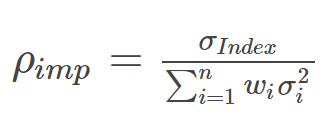
If an index volatility is at 20% and its members average a volatility of 25%, the implied correlation (ρ) might be around 64%. This implies that by selling options in the index and buying the stocks, you’re effectively going short on a correlation of 64%.
Dispersion trading can be profitable, but it’s nuanced and depends on the dynamics of implied and realized correlations in relation to overall market volatility. For instance, in normal conditions, indices like SX5E and S&P500 may have an implied correlation ranging from 50-70% and a realized correlation of 30-60%. This gap reflects the market’s anticipation that extremely low correlations are unlikely to persist, presenting potential risks for a long dispersion trade. The strategy inherently assumes that implied correlation is expected to be above the average realized correlation due to its short volga nature.
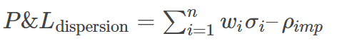
Dispersion trading is sensitive to volatility of volatility, also known as “volga,” due to its reliance on the correlation being linked to volatility. The profitability of a dispersion trade, represented mathematically as P&L of dispersion, can calculated by the sum of the weighted realized volatilities of individual stocks minus the implied correlation of the index which the trader sold, which can be calculated:
Dispersion trading can employ several instruments, with straddle (or call) dispersion being the most liquid and transparent. At-the-money (ATM) straddles are typically used, though trading at 90% strikes can increase the levels of implied correlation sold. However, managing such options positions demands labor-intensive delta-hedging and constant monitoring of vega, a measure of sensitivity to volatility. A lack of vega management can lead to losses, even when the correlation position is correct. Out-of-the-money (OTM) strangles are suggested as an alternative due to their flatter vega profile, although they are less practical for trading.
Example of a Dispersion Trade (NASDAQ-100)
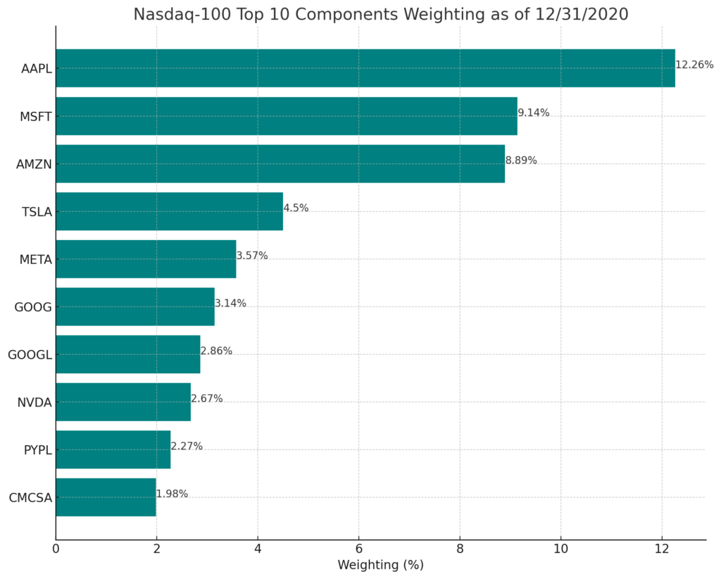
The Nasdaq-100 (NDX) consists of the hundred largest stocks primarily listed on the Nasdaq stock market. This index, being capitalization-weighted, means that larger companies have a greater impact on the daily movements of the NDX. The ten largest NDX components, as listed in the following table, represent about half of the index’s total capitalization, making up 51.42% at the end of 2020. This concentration of a few stocks in the NDX is a key reason why the NDX is an ideal index for executing dispersion trades, as the priced in correlation is relatively high, while the actual realized correlation is relatively low.
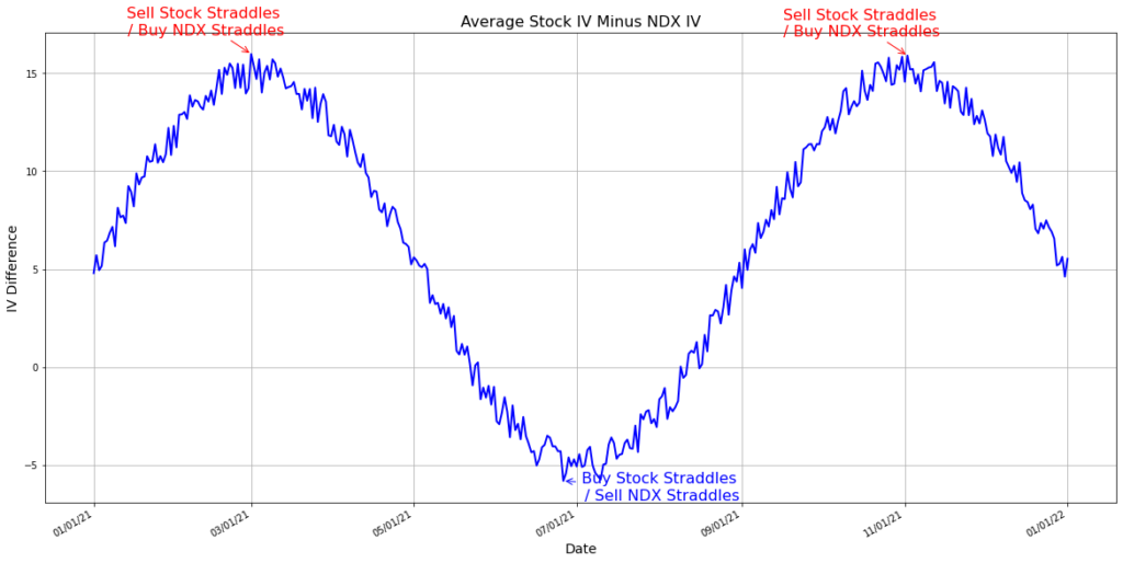
Another aspect for traders to consider in NDX and its major components for dispersion trading is the relationship between volatility expectations. A chart showing the average 30-day at-the-money implied volatility for the top ten NDX components versus the NDX at the end of 2020 reveals that the component volatility, calculated based on market capitalization, is consistently higher than that of the NDX. This difference in volatility presents trading opportunities, as indicated by the chart displaying the spread between the weighted average implied volatility of these top ten stocks and the NDX implied volatility.


In 2021, this spread between individual stock and NDX implied volatility averaged just over 9.00, reaching a high of 18.41 and a low of 4.56. This simple yet effective method of comparing stock and index volatility illustrates the potential trading opportunities in this domain.
Dispersion typically includes taking opposite positions on the volatility of individual stocks compared to the index they belong to, often through at-the-money straddles. Let’s break down the process and provide some illustrative examples.
How to Execute Dispersion Trades:
- Identifying Trade Direction:
- High Spread: If the “Average Stock IV Minus NDX IV” chart indicates a high spread, the trader would likely sell at-the-money straddles for individual stocks and buy at-the-money straddles for the NDX.
- Low Spread: Conversely, if the spread is at the lower end, the trader would purchase straddles for individual stocks and sell an at-the-money straddle for the NDX.
- Determining Portfolio Weighting:
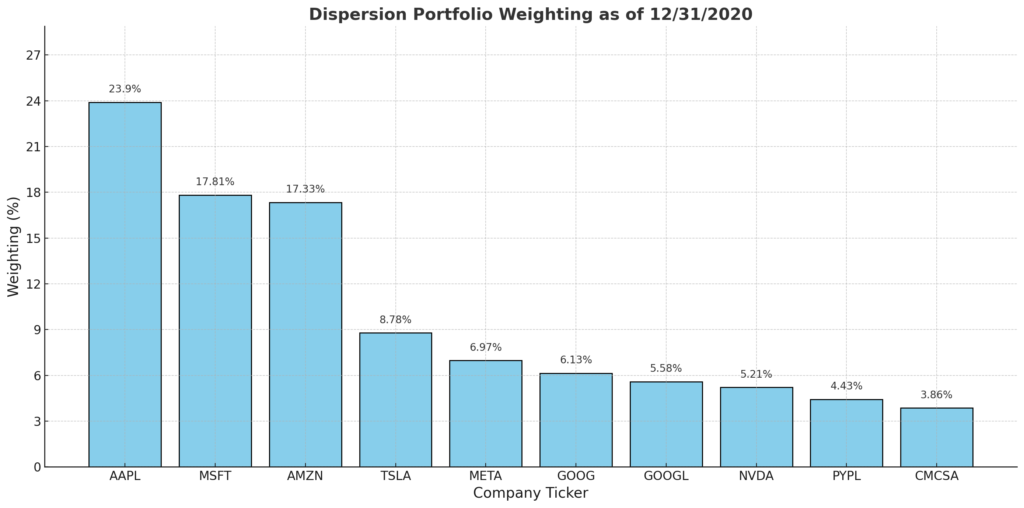
- To set up a dispersion trade, first calculate the weightings of each stock within the portfolio based on their market capitalization as of a specific date (e.g., December 31, 2020).
- Large-cap stocks like Apple, Microsoft, and Amazon may dominate the portfolio. The combined weight of these stocks will dictate the relative number of options to be traded against the NDX options.
- Calculating Number of Options:
- You need to determine the number of options to trade for each stock, which is influenced by the stock’s weighting in the portfolio and the strike price closest to the stock’s current price.
- To ensure a balanced trade that includes options for each stock in the top ten, you might decide to trade a minimum number of NDX straddles. For instance, with two NDX contracts, you’d adjust the number of individual stock options accordingly.
On February 26, 2021, suppose Microsoft (MSFT) closed at $232.38, and the NDX closed at 12909.44. The nearest strike price for MSFT is 232.50, and for NDX, it is 12910. To match the trade with the portfolio’s weighting for MSFT, which is 17.78% at the time (see barchart below), you calculate the number of MSFT straddles to trade against the NDX straddle.
Long Stock / Short NDX Volatility Trade:
- Setting Up the Trade:
- On February 26, 2021, a trader notices the spread between the NDX and individual stock implied volatilities is at the lower end, at 5.31, indicating it might be an opportune time to go long on stock volatilities while shorting NDX volatility.
- Using options that expire on March 26, 2021, the trader buys at-the-money straddles for individual stocks (long position) and sells an at-the-money straddle for the NDX (short position).
- Analyzing the Results:
- As the market closes on March 26, the trader reviews the outcome. The long positions on individual stocks are not profitable except for Meta Platforms, Inc. (previously known as Facebook). Despite this, the short position on the NDX straddle is profitable enough to offset the losses from the individual stocks, resulting in a net profit.
- Capitalizing on Volatility Spreads:
- On April 16, 2021, the spread between stock and NDX volatility is much higher, at 13.25. In this scenario, the trader does the opposite by purchasing an NDX straddle and selling straddles on the individual stocks.
- This trade turns out to be profitable on both ends, with the long NDX straddle and the short positions on the equity straddles yielding a combined gain.
The date on the “Average Stock IV Minus NDX IV” chart, April 16, 2021, shows a notable spread of 13.22 between the portfolio’s implied volatility and that of the NDX, which is toward the upper limit of its range. On this occasion, a strategy was employed where an NDX straddle was bought while selling straddles on the individual stocks. The outcome of this strategy was quite favorable; both the long position in the NDX straddle and the short positions in the equity straddles yielded profits. The cumulative gain at the expiration of all options stood at 554.23.
The timing strategy for the above dispersion trades relies on the comparison between the implied volatilities of a stock portfolio akin to the index, though it is not the sole method for initiating dispersion trades. There are numerous, more intricate strategies for dispersion trading, and it is uncommon to hold these positions until expiration. Nonetheless, the cases presented in this discussion illustrate the trading of volatility discrepancies between stocks and an index. The Nasdaq-100 market, dominated by a handful of stocks, presents an especially suitable environment for dispersion trading strategies.
Considerations in Dispersion Trading
The Greeks, or the risk measures of dispersion trading, depend heavily on how the vega (volatility exposure) is weighted across its components.
In vega-weighted dispersion, which balances the vega of the short index and long single-stock positions, the trade inherently has zero vega. However, it typically carries short positions in both gamma (rate of change in delta with the underlying) and theta (time decay).
For a theta-weighted dispersion trade, the size of the long single-stock leg is smaller than the index leg. This sizing aims to balance the theta paid on the long single-stock leg with the theta earned from the short index leg. As a result, a theta-weighted dispersion is significantly short in gamma, even more so than a vega-weighted dispersion.
Conversely, gamma-weighted dispersion necessitates a larger long single-stock leg compared to the index leg, enhancing gamma exposure but also increasing the theta paid. This trade-off makes gamma-weighted dispersion less commonly used.
Dispersion can be weighted according to theta, vega, and gamma. Each weighting has implications for the trade’s exposure to correlation. Theta-weighted dispersion, in particular, offers a nearly pure correlation exposure, with its profitability largely hinging on the difference between realized and implied correlations. For investors, the timing of entry points in theta-weighted dispersion should consider the implied correlation of the index.
Vega-weighted dispersion, combining elements of theta-weighted dispersion and a long single-stock volatility position, provides a hedged exposure to mispricing in correlation. This strategy’s effectiveness depends on the gap between average single-stock volatility and index volatility, and it’s generally seen as providing greater exposure to correlation mispricing.
Gamma-weighted dispersion, while theoretically sound, is rarely used in practice due to its demanding requirements and the typically higher implied volatility of single stocks compared to indexes.
In summary, dispersion trades are short vol of vol (volatility of volatility, or volga). The profit and loss (P&L) of a theta-weighted dispersion trade is tied to the difference between implied and realized correlations, adjusted by a factor representing the weighted average variance of the index’s components. As both volatility and correlation tend to increase during market downturns, the payout of a dispersion trade is impacted by these changes, making the strategy inherently short in volga.
Additional factors to take into account when engaging in dispersion trading include:
- Portfolio Weighting: It’s critical to determine the weight of each stock in your portfolio based on its market cap. For the top constituents like Apple, Microsoft, and Amazon, which make up a significant portion of the portfolio, you’ll need to decide how many options to buy or sell for each, relative to their weighting.
- Timing and Methodology: While the examples provided are based on observing implied volatility spreads, it’s worth noting that there are various complex methods to time dispersion trades. Traders typically don’t hold these positions until expiration due to the dynamic nature of the markets.
- Market Suitability: Given that a few stocks often comprise a substantial portion of an index like the Nasdaq-100, it becomes an ideal market for implementing dispersion trades. This allows traders to leverage the outsized influence of these stocks on the index’s performance.
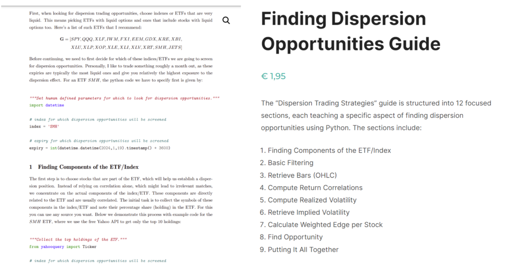
For a full guide on dispersion trading including Python code snippets. I recommend checking out our full guide. Just as a teaser we also show you a glimpse of the current best dispersion opportunities for the ETFs: SPY,QQQ and XLF in the green table below.
Dispersion Trading Opportunities
Recommended Reading
- [1]: S&P U.S. Indices Methodology – S&P Dow Jones Indices.
- [2]: Volatility Dispersion Trading – Q. Deng, University of Illinois at Urbana-Champaign.
- [3]: Volatility and Correlation: The Perfect Hedger and the Fox – Riccardo Rebonato.
- [4]: Option Volatility & Pricing: Advanced Trading Strategies and Techniques – Sheldon Natenberg.
- [5]: Trading Options Greeks: How Time, Volatility, and Other Pricing Factors Drive Profits – Dan Passarelli.
- [6]: Dynamic Hedging: Managing Vanilla and Exotic Options – Nassim Nicholas Taleb.
- [7]: Volatility Trading – Euan Sinclair.
- [8]: The Concepts and Practice of Mathematical Finance – Mark S. Joshi.
- [9]: Analysis of Financial Time Series – Ruey S. Tsay.
- [10]: Quantitative Trading: How to Build Your Own Algorithmic Trading Business – Chan, E.P.
- [11]: Option Volatility and Pricing – Sheldon Natenberg.
- [12]: Understanding Volatility Smile – Investopedia.
- [13]: Advances in Financial Machine Learning – Marcos Lopez de Prado.
- [14]: Margin Requirements for Option Writers – Investopedia.
- [15]: Wikipedia on Dispersion Trading – Wikipedia
- [16]: Wikipedia on Correlation Trading – Wikipedia
- [17]: Quora on Dispersion Trading – Quora
- [18]: Github on Dispersion Trading – Github
- [19]: Huggingface – Readme
- [20]: Samsung
- [21]: Dispersion Trading – Medium